모델을 학습하려면?
주어진 것:
- 모델: \( f_{\theta}(x) \) (MLP - 다층 퍼셉트론)
- 데이터 세트 \( D \): \(\{(x^{(1)}, y^{(1)}), (x^{(2)}, y^{(2)}), \ldots, (x^{(N)}, y^{(N)})\}\)
필요한 구성 요소:
- 모델의 파라미터 \( \theta \)
- cost 함수
- Gradient Descent
- Backpropagation
Loss function, Cost function
대표적으로 MSE
\[ L(\theta) = (f_{\theta}(x) - y)^2 \]
샘플당 모델 예측값, ground truth 의 차이
Cost 함수는
\[ J(\theta) = \frac{1}{2N} \sum_{i=1}^N (f_{\theta}(x^{(i)}) - y^{(i)})^2 \]
이 식을 최소화하는 \theta 찾는게 목표
그러기 위해 이용하는게
Gradient Descent
\[ \theta_j := \theta_j - \alpha \frac{\partial J(\theta)}{\partial \theta_j} \]
여기서 \( \alpha \)는 learning rate.
j 번쨰 파라미터에서 편미분해서 기울기 구하고 기울기의 반대방향으로 가야하는거니까 마이너스를 붙여서 가주면 됨.
Backpropagation
- Backpropagation이란 실제값과 예측값의 에러를 모델의 각 파라미터들로 전파시켜 업데이트 하는 방법
- 각 파라미터의 기여도, 즉 에러를 내는데 얼마나 기여했는지 에 따라 업데이트됨
Backpropagation 예시
아래 그림은 Backpropagation 과정의 예시를 대충 그려봤는데
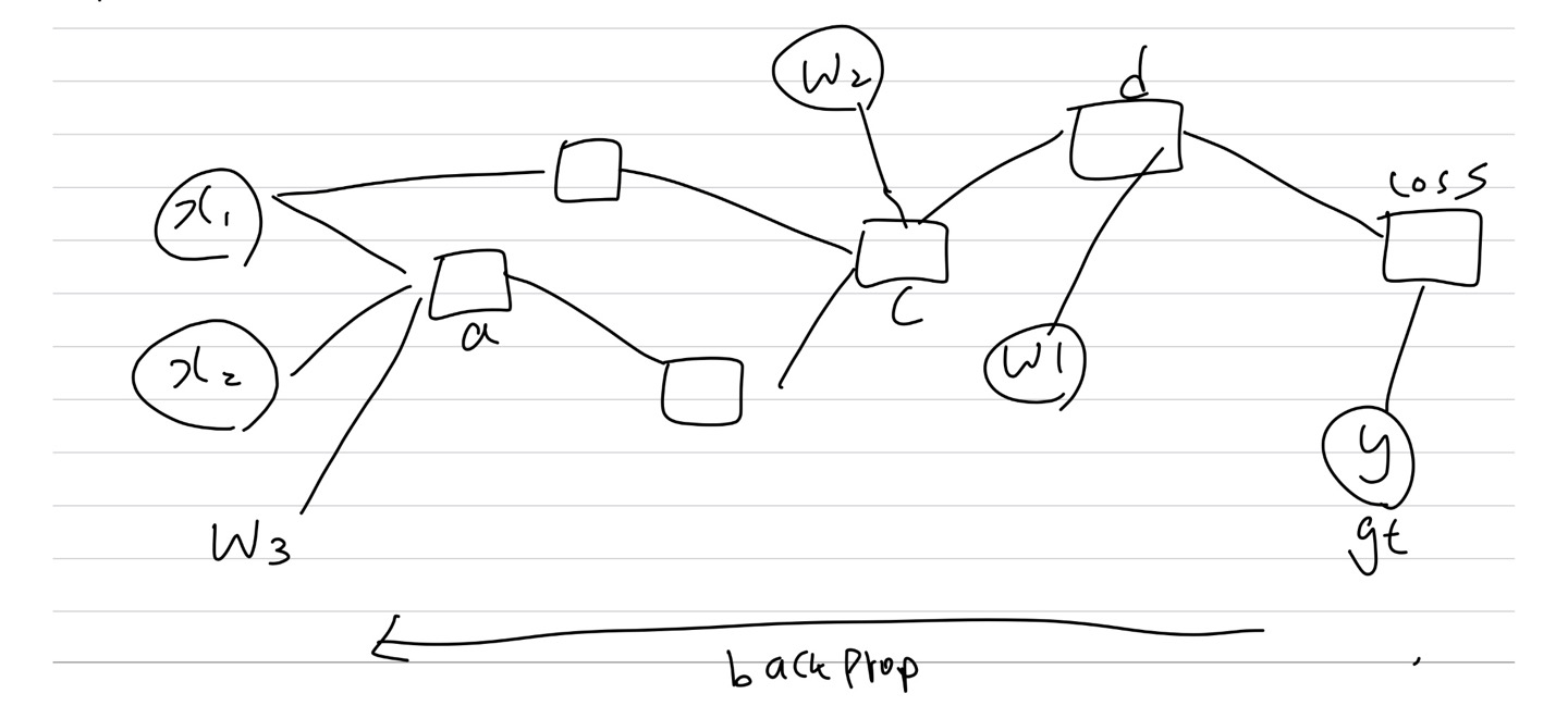
여기서 각 노드들의 의미가
- \(x_1, x_2\)는 입력 값
- \(a, b, c, d\)는 각 레이어의 뉴런 값
- \(w_1, w_2, w_3\)는 가중치
- Loss는 손실 함수
Chain Rule
기울기를 계산하기 위해 Chain Rule을 사용함.
\[ \frac{\partial \text{Loss}}{\partial w_1} = \frac{\partial \text{Loss}}{\partial d} \cdot \frac{\partial d}{\partial w_1} \]
\[ \frac{\partial \text{Loss}}{\partial w_2} = \frac{\partial \text{Loss}}{\partial d} \cdot \frac{\partial d}{\partial c} \cdot \frac{\partial c}{\partial w_2} \]
\[ \frac{\partial \text{Loss}}{\partial w_3} = \frac{\partial \text{Loss}}{\partial d} \cdot \frac{\partial d}{\partial c} \cdot \frac{\partial c}{\partial b} \cdot \frac{\partial b}{\partial a} \cdot \frac{\partial a}{\partial w_3} \]
여기 마지막에서 의미를 좀 해석해보면, w3이 얼만큼 loss 에 기여했는지 한번에 미분이 안되니까 c가 d에 미치는 영향, b가 c에 미치는 영향 ~~ 쭉쭉 구해서 결국 w3이 loss에 비치는 영향까지 알수 있는것임.
이런 계산은 사실 computation graph 같은거 이용하면 한번에 쉽게 구할수 있는데 이 내용은 우선 넘어가겠음. 궁금하면 다른 블로그 [CS224N] Lecture 4: Back Propagation and Computation Graphs (velog.io)
[CS224N] Lecture 4: Back Propagation and Computation Graphs
작성자 : 16기 이승주
velog.io
여기 참고하면 될듯!